Data wrangling & manipulation in R - workshop site

Day 1 notes: Tidy data principles & tidyr

Ruan van Mazijk

Introducing Ruan

• BSc + Hons here at UCT

• Ecology & evolution
• (Mostly plant) comparative biology

• Biogeography

• Been working with R for 4.5 years

• Every major project I’ve done…

• My MSc is on the relationships between genome-size and plant phenotypes and ecology in CFR Schoenus and Tetraria species (Cyperaceae, tribe Schoeneae)

Workshop goals

• More reproducible science
• Save time by:
  • Automating repetitive tasks
  • Eliminating human error
• Boost your skills
• Think about your data programmatically

Workshop outline

Day	Topic
1	Tidy data principles & tidyr
2	Manipulating your data & an intro to dplyr
3	Extending your data with mutate(), summarise() & friends

But before that, we need to discuss something technical…

The 2 dialects of R

1. base
   • $, [], [[]], apply(), which(), subset()
2. tidyverse
   • What we are going to learn in this workshop

The base way of doing things can sometimes lead to messy R-scripts:

data <- read.csv("my-data.csv")

data1 <- f(data, arg1 = "something")
data2 <- g(data1, another.thing = "blah")
data3 <- h(data2, a.setting = TRUE)
data4 <- data3[data3$a.column == "cough", ]

Look at all those intermediate objects we don’t care about :cold_sweat:

Or, worse, if we try to remove the intermediate objects, we get hard to read code:

data <- read.csv("my-data.csv")

data <-
  h(
    g(
      f(
        data,
        arg1 = "something"
      ),
      another.thing = "blah"
    ),
    a.setting = TRUE
  )

data <- data[data$a.column == "cough", ]

And we still can’t get rid of that subsetting line easily!

The solution? A handy addition to normal R-syntax: the “pipe” %>% (also pronounced “then”).

With the pipe, we feed the result of one line of R-code into the next (i.e. we send the result of one expression to the next):

f(x)
x %>% f() # same thing

This allows us to compose functions really easily!

Instead of this mess:

h(g(f(x)))

We can do this:

x %>%
  f() %>%
  g() %>%
  h()

Much easier to read! Instead of reading from the inside-out, we can read top-to-bottom :smiley:

A motivating example

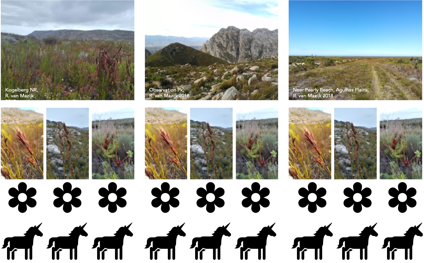
An example data-collection scenario in biology

Collecting your data like this is fairly practical!

One way to lay out your collected data…

But computers will struggle to use this, and so will you, to answer questions about pollinator vs flower abundance!

Another way…

The “best” way. (Will make your life easiest in the long-term.

This is tidy data. Moreover, tidy data is defined as follows:

1. Each variable must have its own column.
2. Each observation must have its own row.
3. Each value must have its own cell.

(Image CC BY-NC-ND 3.0 Grolemund & Wickham 2017, R for Data Science)

How do we get our data to look this way?

tidyr

An R-package all about getting to this:

tidyr provides us with:

Verbs to tidy your data

# Untidy observations?
gather()    # if > 1 observation per row
spread()    # if observations live in > 1 row

# Untidy variables?
separate()  # if > 1 variable per column
unite()     # if variables live in > 1 column 

Note the following when choosing tidyr:: verbs

• Be clear on what your observations are
  • Like, what unit of your study counts as an observation
  • E.g. Leaf traits: plant leaf vs plant individual
  • E.g. Reproductive success: egg size vs clutch size
  • This will depend on your study &/or data!
• Variables are discrete, seperate ideas

Untidy observations?

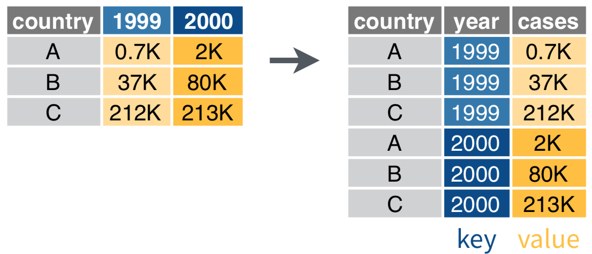
Use gather() if > 1 observation per row

data %>%
  gather(key, value, ...)

data %>%
  gather(key = year, value = cases, `1999`, `2000`)

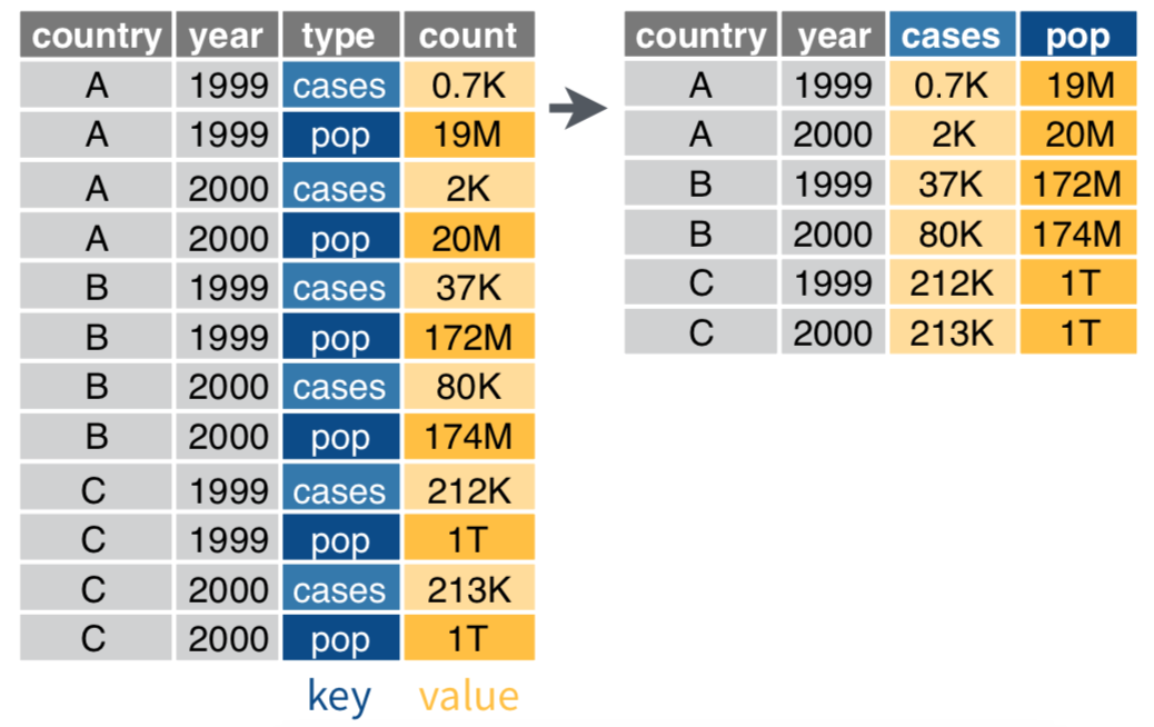
Use spread() if observations live in > 1 row

data %>%
  spread(key, value)

data %>%
  spread(key = type, value = count)

Untidy variables?

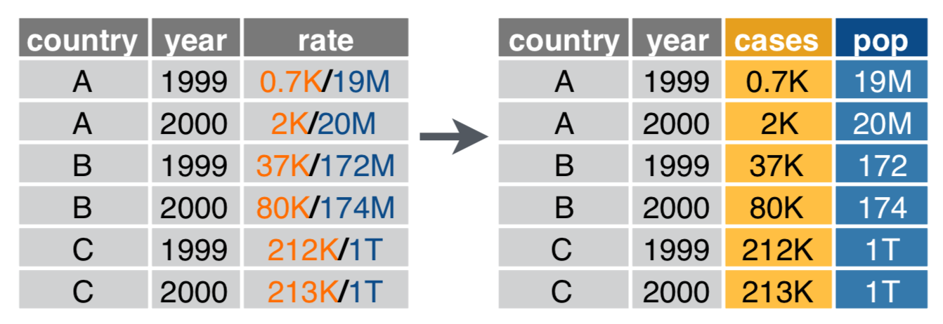
Use separate() if > 1 variable per column

data %>%
  separate(col, into, sep)  # sep's default is any non-alphanumeric character

data %>%
  separate(col = rate, into = c("cases", "pop"))

Use unite() if variables live in > 1 column

data %>%
  unite(col, ..., sep)  # again, sep's default is any non-alphanumeric character

data %>%
  unite(col = year, century, year)

---

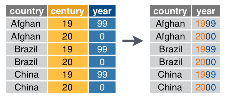
Diagrams illustrating gather(), spread(), separate() and unite() are taken from RStudio cheatsheets (CC BY SA RStudio)

This site is open source. Improve this page.